AN1: Impedance Measurement Accuracy and Influencing Factors

Scope

This note explains how to reach and extend high impedance measurement accuracy by choosing appropriate cabling, for the CI Impedance EIS and CI Impedance EIT device for two measurement mode

• EIS, 2- or 4-electrode : direct impedance measurement
• EIT "custom" : multiplexed impedance measurement across N electrodes (multi-spectroscopy combined), N=12 in the reference configuration

Both modes share the same underlying model, with EIT custom simply calling for tighter cable capacitance to reach the same accuracy, since its multiplexed topology combines more channels on the same cable.

CI Impedance EIT itself can be operated in two distinct modes: standard EIT, which reconstructs from relative measurements against a reference state and is, by construction, only weakly affected by external factors such as cable capacitance; and EIT "custom", covered in this note, where individual channel combinations are read out directly and are therefore sensitive to the same parasitic-capacitance mechanism as EIS. Standard EIT is out of scope here — its relative-reconstruction approach already delivers high accuracy across a wide range of cabling

Part 1 : In practice

Where the capacitance comes from

The internal connectivity (multiplexer + M12 connector) contributes a small, well-controlled baseline, characterized in-house and already folded into every chart in this note, present even before any external cable is attached. On top of this excellent baseline, the cable is the one element the user can choose freely to reach a target accuracy, and the right choice can extend the usable range considerably.

Actual cable capacitance depends heavily on construction (wire gauge, spacing, shielding, length), so the table below gives illustrative examples rather than a fixed specification. It's meant to build intuition for the order of magnitude at stake, not to replace characterizing the specific cable in use.

Example cable	Typical capacitance observed	What drives it
Individually-shielded conductors (e.g. microcoax), each shield grounded	~1 pF (cable only)	Each signal's field terminates on its own local shield instead of reaching neighboring conductors
TouchProof-type cable	~15 pF (cable only)	Typical EIS 2/4-electrode cable
Button cable, separated wires	~18–20 pF/m	Wires kept apart, limited coupling
Button cable, twisted/bundled wires	~30–34 pF	Wires close together, increased coupling
M12 ribbon cable, 1 m	~75 pF (total, incl. internal)	12 conductors in the same jacket
M12 ribbon cable, 2 m (current)	~136 pF (total, incl. internal)	Linear capacitance ≈ 60 pF/m
Single overall shield around the whole bundle, grounded	Little to no improvement over the unshielded value above	Blocks external interference, but conductors inside the shield remain coupled to each other almost as much as without it
Any shielded cable, shield not grounded	Same as unshielded cable (often >80 pF/m)	Shielding only works once grounded

Achievable accuracy charts

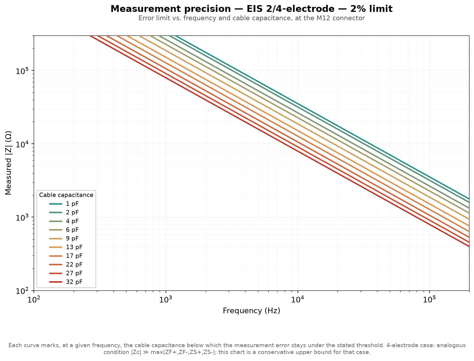
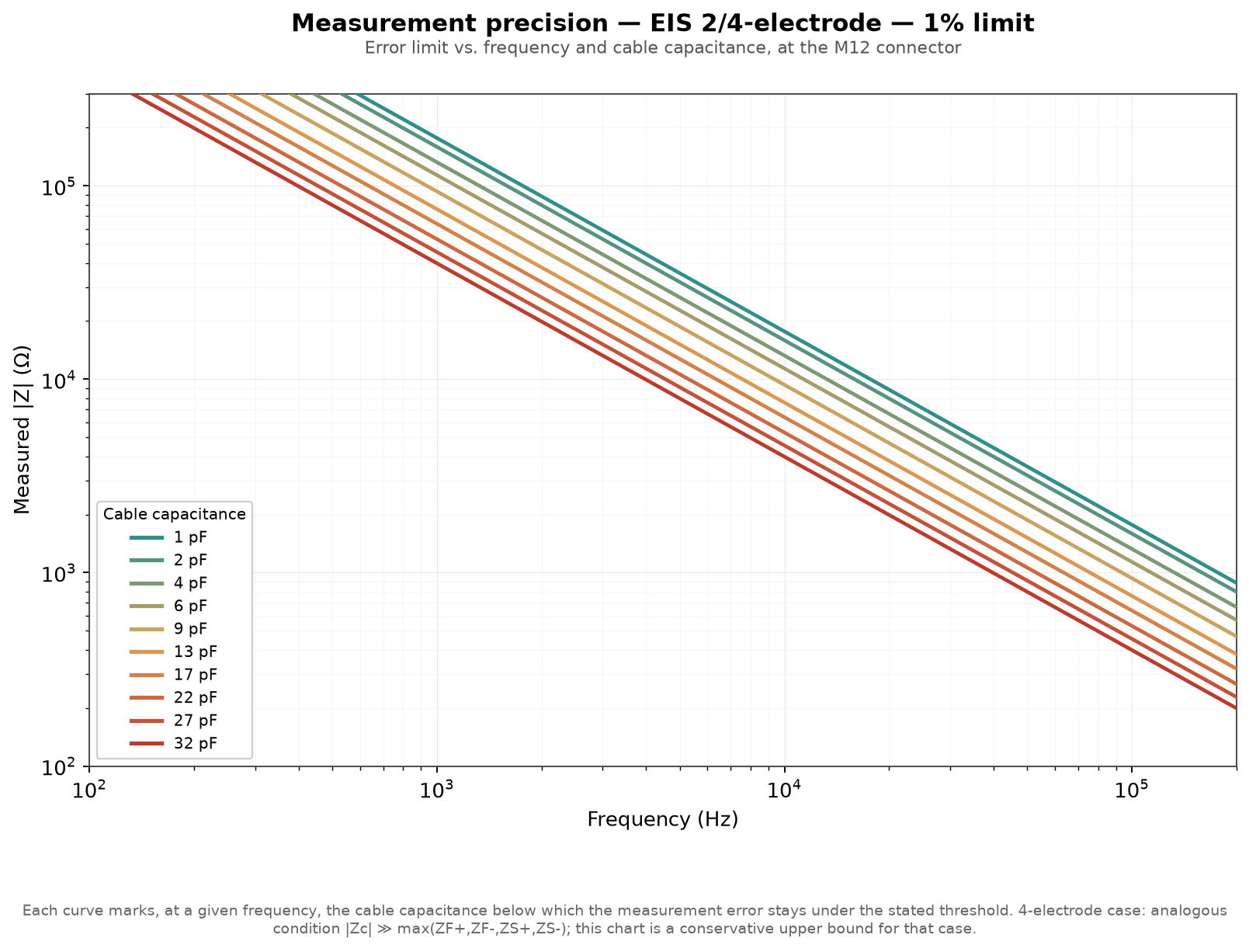
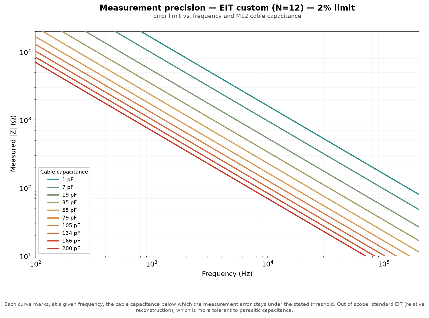
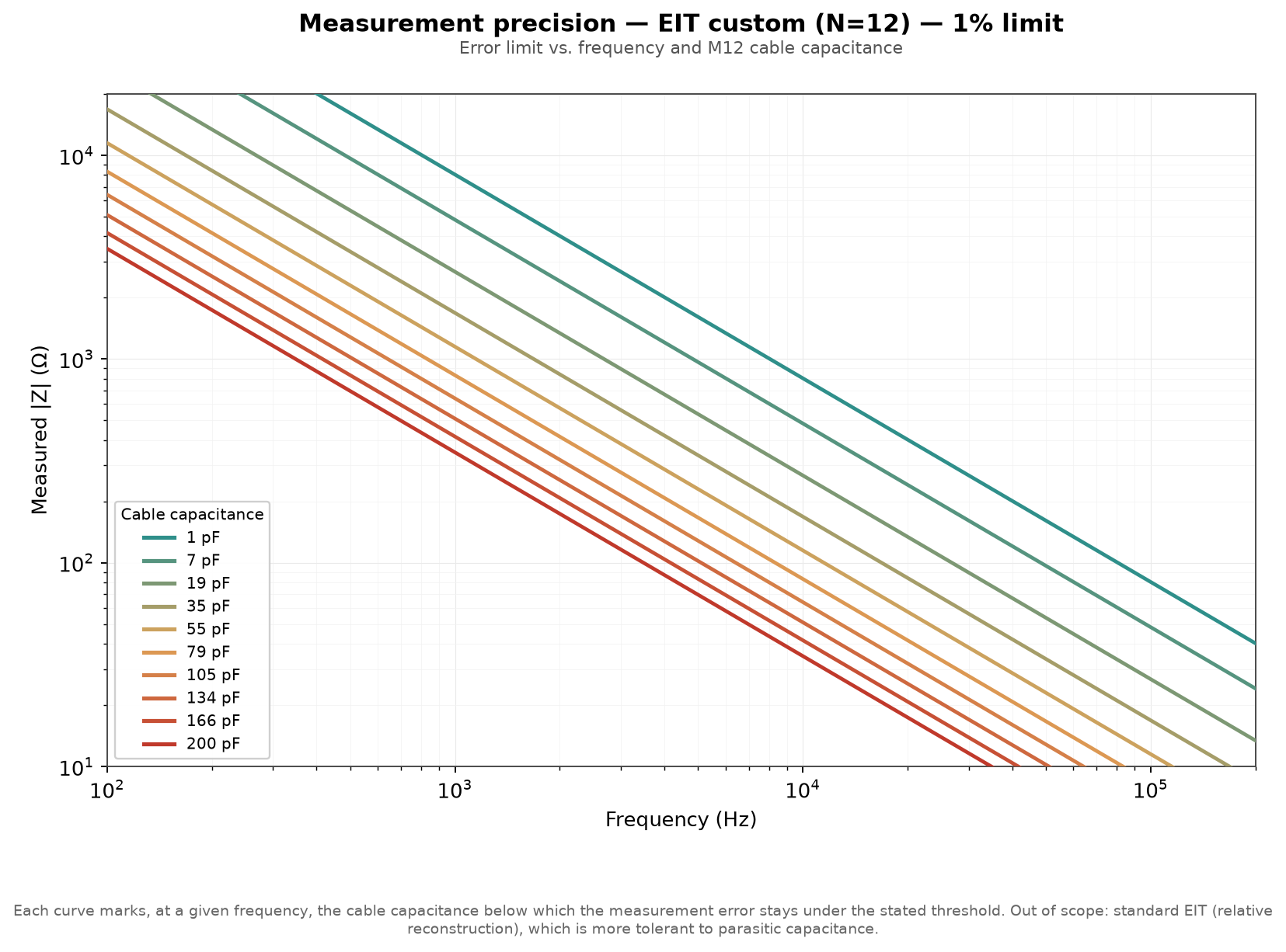
The four charts below help evaluate how to stay under a 1% or 2% error, as a function of frequency and cable capacitance (the internal baseline is already included in the underlying calculation). Each curve marks, at a given frequency, the cable capacitance that keeps the measurement within the stated accuracy.

CI Impedance EIS, 2/4-electrode

CI Impedance EIT, custom (N=12)

Recommendations

• Always characterize your own cable capacitance rather than assuming a nominal value. Connector type, wire routing, and length all shift it, sometimes considerably.
• Always evaluate the electrode-skin (or electrode-medium) contact impedance for your specific application. It adds directly to the impedance the system sees, and in 4-electrode/EIT custom it also governs how tightly the |Zc| ≫ max(...) condition is met: a high-contact-impedance electrode can dominate the achievable accuracy even with an excellent cable.
• Design with a margin: so that real-world accuracy stays comfortably under 1% once second-order effects (capacitance asymmetry, contact impedance variability, reconstruction residuals in the multiplexed case) are folded in. The approximation Ɛr ≈ |Z|/|Zc| is excellent well below this margin, and becomes conservative to trust as the ratio |Z|/|Zc| approaches 0.5.

Extending accuracy further

Beyond the cables covered above, individually-shielded conductors, with each shield grounded, are available as an option (e.g. microcoax per channel) and have been validated experimentally: this brings cable capacitance down to approximately 1 pF (vs. ~15 pF for a standard EIS cable, or ~60 pF/m for the current unshielded EIT ribbon cable), extending the usable frequency and impedance range well beyond the standard specification.

Two conditions matter for this to work: the shield must be grounded, and it must enclose each conductor individually, not just the cable bundle as a whole. A single overall shield around the whole bundle mainly blocks external interference; it does little to reduce the capacitive coupling between the conductors it encloses, which is the mechanism this note addresses. It still has real value, though: by removing the cable's sensitivity to its environment (nearby objects, movement, EMI), it makes the parasitic capacitance more stable and repeatable from one measurement to the next, even though its average value stays close to the unshielded case.

This option is available on request for applications that call for a wider frequency range or higher measurable impedance at a given accuracy target, in either EIS or EIT custom mode.

Part 2 : Theory

2-Electrode Measurements

In the case of a 2-electrode measurement, the influence of the cables and the multiplexer can be modeled as follows:

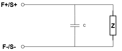
Instead of the capacitance (C), it would be possible to introduce a complex impedance to more faithfully represent the actual behavior of the system. However, given the frequency range used as well as the various characterization tests performed, it is reasonable to consider that this behavior can be approximated by a capacitor.

The measurement error then arises from the fact that the system measures the equivalent impedance (Z // Z_c) instead of the actual impedance (Z). The impact of this error depends directly on the respective values of (Z) and (Z // Z_c).

The relative measurement error can thus be written as:

Ɛr = |(Z // Z_c - Z)| / |Z| = |Z| / |Z + Z_c|

We can assume that: |Z_c| >> |Z|. Indeed, in the opposite case, the error would exceed 50%, which corresponds to a situation far removed from normal sensor operating conditions.

Under this assumption, the previous expression can be simplified to:

Ɛr ~= |Z| / |Z_c|

This means that, to guarantee an error of less than 1%, it is necessary to measure impedances satisfying:

|Z(f)| < 0.01|Z_c|

Where:

|Z_c| = 1 / (2 π f C)

We therefore obtain, for a given frequency (f):

|Z(f)| < 0.01 / (2 π f C)

This relationship defines the maximum measurable impedance limit in order to keep the error induced by the parasitic capacitance below the 1% threshold.

**Caution :** This measurable impedance limit corresponds to the total impedance seen by the measurement system. It therefore includes not only the impedance of the medium being studied, but also the electrode-skin contact impedance, which can in some cases represent a significant contribution to the total measured impedance.

4-Electrode Measurements

In the case of a 4-electrode measurement, the equivalent schematic becomes noticeably more complex:

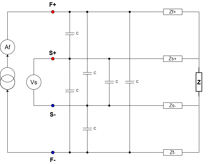
where:

• Z represents the impedance to be measured;
• Z_F+, Z_F-, Z_S+ and Z_S- represent the electrode-skin contact impedances;
• C represents the parasitic capacitance introduced by the cables and/or multiplexers.

As might be expected, the analysis here becomes considerably more complex than in the case of the 2-electrode measurement.

The impedance is measured from the ratio: Z = V_S / A_F

However, it immediately becomes apparent that the current flowing through impedance Z is not necessarily equal to the measured current (A_F), just as the measured voltage (V_S) is not necessarily equal to the voltage actually present across the terminals of Z.

Consider for example the following diagram:

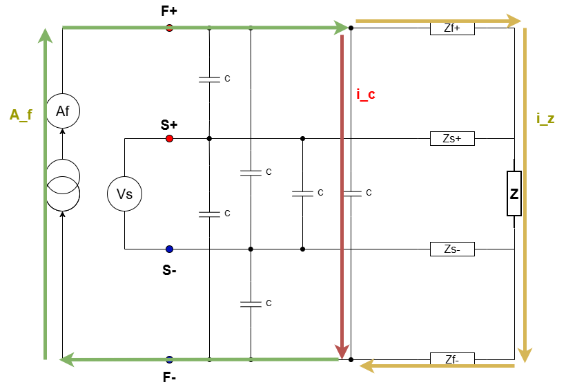
Focusing solely on the current paths indicated above, we observe that a leakage current flowing through the parasitic capacitance between F+ and F- can disturb the measurement of the injected current.

In this case, A_F = I_C + I_Z, whereI_C corresponds to the leakage current flowing through the parasitic capacitance and I_Z to the current flowing through the measured impedance.

A correct measurement is obtained only if |Z_C| >> |Z_F+ + Z_F- + Z| because this condition guarantees that I_C << I_Z , and therefore that the influence of the parasitic capacitance remains negligible.

This parasitic capacitance can also affect the voltage measurement.

Now consider the current paths shown in the following diagram:

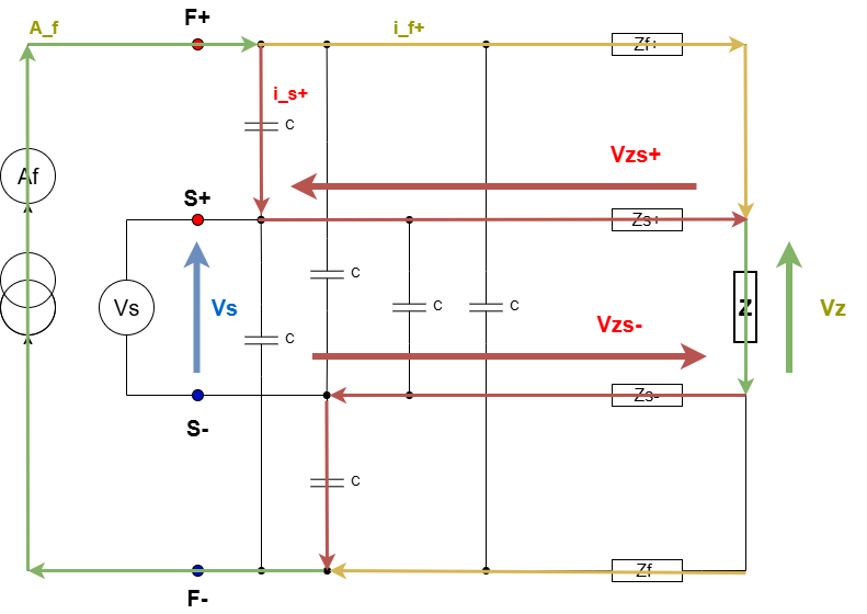
We then observe that the measured voltage becomes V_S = V_Z + V_Zs+ + V_Zs-

In this case, the error appears when the voltage drops across the contact impedances V_Zs+ and V_Zs-become of the same order of magnitude as the voltage measured across the impedance of interest (Z).

To limit this effect, it is necessary to impose: |Z_C| >> |Z_S+| (an analogous reasoning also applies to Z_S-)

This condition ensures that the voltage divider formed between Z_S+ and Z_C does not significantly influence the measured voltage.

All of these effects remain difficult to predict analytically, as they depend heavily on the electrode-skin contact impedance, and therefore directly on the type of electrode used as well as its positioning.

Furthermore, asymmetries between the parasitic capacitances associated with each electrode, or differences between the contact impedances (Z_F+, Z_S+,etc.), can also introduce additional filtering effects likely to distort the results.

It is therefore strongly recommended to maximize the equivalent parasitic impedance Z_C, that is, to minimize the parasitic capacitance C as much as possible.

In practice, if we ensure that: |Z_C| >> max( Z_F+, Z_F-, Z_S+, Z_S- ) then all of the error sources previously described become negligible, thereby making it possible to obtain a reliable and robust measurement.

Custom EIT Measurements

The case of custom EIT is considerably more complex, because each channel shares a parasitic capacitance with all the other channels connected to the same cable or the same multiplexer. It is therefore necessary to analyze this case in more detail.

The equivalent schematic of a "custom" EIT measurement is as follows:

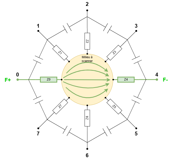
Here, 0, 1, ..., N represent the different channels — or electrodes — among which the F+, F-, S+, S- signals can be multiplexed.

The impedances Z₀, Z₁, ..., Z_N correspond to the electrode-skin contact impedances of each electrode, while the capacitors represent the parasitic capacitances between cables.

It should be noted that this schematic remains simplified. In reality, a parasitic capacitance exists between every pair of electrodes (between 1 and 3, between 1 and 4, etc.), and not only between consecutive electrodes.

As in the case of the 4-electrode measurement, the system is too complex to allow a complete analytical analysis. We will therefore reason based on the current paths observed in the measurement.

Ideally, the current distribution is the one shown in the previous figure. If a current is injected between electrodes 0 and 4, the entire current first flows through Z₀, then circulates through the medium following the most favorable impedance paths, and finally exits entirely through electrode 4 by flowing through (Z₄).

From this current distribution in the medium, the relevant potential differences are then measured.

In the case of standard EIT, these voltages would be measured between all electrodes except those used for current injection (here 0 and 4). However, the custom EIT mode also allows configurations equivalent to 4-electrode or even 2-electrode measurements, with any electrode configuration set by the user.

In reality, the presence of parasitic capacitances disrupts this ideal current distribution, as illustrated below:

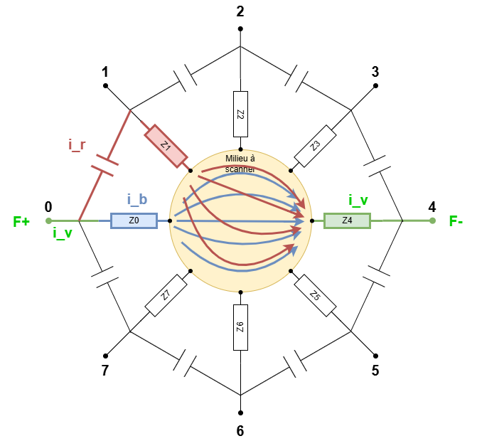
We observe that the parasitic capacitance between electrodes 0 and 1 creates an alternative path for the current. Instead of following the normal route: Z₀->medium -> Z₄, part of the current can take the following path: Z_C -> Z₁ -> milieu -> Z₄. The essential question then is to determine to what extent this parasitic current introduces a significant error.

Since both paths share the same potential at electrode 0 as well as at Z₄, we can write:

i_B ( Z₀ + Z_0-4 ) = i_R ( Z_C + Z₁ + Z_1-4 )

where:

• i_B represents the current following the intended path;
• i_R represents the leakage current taking the parasitic path.

We can then define the relative error as:

Ɛr = i_R / i_B = ( Z₀ + Z_0-4 ) / ( Z_C + Z₁ + Z_1-4 )

As in the previous case, we can assume:

|Z_C| >> |Z₁ + Z_1-4|

Indeed, if this condition were not satisfied, the error would exceed 50%, making the measurement of little use.

We then obtain the approximation:

Ɛr ~= ( Z₀ + Z_0-4 ) / Z_C

The conclusion here is similar to the case of 2-electrode measurements:

• the higher the parasitic capacitance C, the lower the capacitive impedance Z_C, which increases the error;
• the higher the contact impedance of the injection electrode, the greater the error also becomes.

Two practical conclusions can be drawn:

• it is necessary to minimize the parasitic capacitance introduced by the cables and multiplexers as much as possible;
• the choice of electrodes plays a critical role: the use of dry electrodes, characterized by a higher contact impedance, will lead to a significant increase in measurement error.

Controlling the contact impedance of the electrodes is therefore essential for obtaining reliable results.

However, this analysis remains simplified. In reality, parasitic capacitances exist between all pairs of electrodes: between 0 and 2, between 0 and 3, etc. There is therefore not a single leakage current i_R, but as many leakage currents as there are connected electrodes.

Furthermore, on the F- side (electrode 4 in the example), exactly the same phenomenon occurs: the parasitic capacitances also create multiple alternative leakage paths.

The influence of the parasitic capacitances on the F+ side can thus be represented as follows:

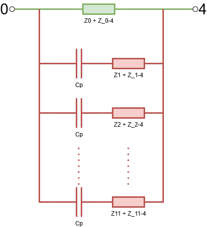
In other words, instead of having a single alternative path for the current, we obtain 11 here, since the cables and multiplexers simultaneously carry 12 signals each.

The same phenomenon occurs on the F- side, creating 11 additional paths this time.

In total, in the worst-case scenario, that is, when: Z >> Z_0, Z_1, Z_2, ..., the simplified equivalent circuit associated with the current injection error can be represented as follows:

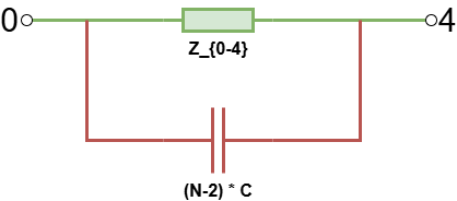
In this case, similarly to the 2-electrode measurement case, the maximum error can be approximated by:

Ɛr ~= |Z| / |Z_c|

with, however, an important difference: here, Z_c no longer corresponds to the impedance of a single parasitic capacitance, but to the equivalent of 22 capacitances in parallel.

We therefore obtain:

|Z_c| = 1 / (44 π f C)

This means that, to guarantee an error of less than 1% in EIT mode, the following condition must be met:

|Z(f)| < 0.01 / (44 π f C)

We can therefore see that custom EIT is particularly sensitive to parasitic capacitances. The multiplication of leakage paths induced by the multiplexed architecture makes this measurement mode much more demanding than the 2- or 4-electrode configurations.

Reducing parasitic capacitances as well as rigorously controlling electrode-skin contact impedances therefore constitute major constraints for ensuring reliable measurements.

Standard EIT Measurements

In the case of standard EIT measurements, the errors introduced by parasitic capacitances are generally less problematic than in the case of custom EIT. This is mainly explained by the fact that the reconstruction algorithms used in tomography are largely based on a relative approach, meaning they compare the acquired measurements to a previously recorded reference state rather than directly using absolute impedance values.

This approach offers an important advantage: the static contributions of the measurement system, and in particular the electrode-skin contact impedances, are largely incorporated into this reference measurement. Their direct influence on the final reconstruction is therefore significantly reduced, which overall makes the system more tolerant of certain hardware imperfections.

However, this approach does not necessarily compensate for all the sources of error described in this document. In particular, phenomena related to leakage currents induced by parasitic capacitances, changes in the distribution of the injected current in the medium, or filtering effects caused by asymmetries between electrodes can still degrade the quality of the acquired data and, consequently, degrade the tomographic reconstruction.

These limitations are particularly significant in biological applications, where the impedance variations to be detected are often small and where the stability of the measurement chain plays a critical role.

For more information, the following paper presents in more detail the main challenges related to impedance tomography applied to biological systems:

Robust electrical impedance tomography for biological application: A mini review - ScienceDirect